The Philosophical Gourmet Report (PGR) is a data resource for prospective graduate students in philosophy to help students choose which graduate programs to pursue. Based on survey data collected from philosophers, the report offers scores and rankings of philosophy PhD-granting Institutions throughout the English-speaking world. To help improve the PGR’s accessibility and impact, I’ve utilized some data analytics methods to create visualizations, analyses, and a relational database for all publicly available PGR data. On this page, I’ll document my process of creating the PGR Database that I’ll use for my analyses and visualizations. To view my findings and analyses, see the main project page for my Data Analysis of the Philosophical Gourmet Report (PGR).
I came up against the limits of using Tableau and Excel alone upon creating dashboard visualizations of the PGR’s speciality scores. In particular, having multiple Excel workbooks hundreds of duplicate strings and sheets leads to cumbersome navigation and makes further analysis difficult. This framework would also demand a substantial amount of work in order to insert and relate data from previous iterations of the PGR. Tableau can definitely handle a full-on relational database, but I have to build it first.
A relational database can efficiently store all the publicly available PGR data while also making it easy to access and visualize without tripping over hundreds of rows of duplicate strings across multiple spreadsheets. The end goal of this project is to design and create a relational database with all the relevant tables and scores over the years for easy querying and visualization. This will be the home page of the database creation project, where I will introduce the project details and thought process, link to the relevant resources (e.g., Github), and document the process.
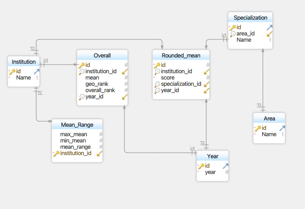
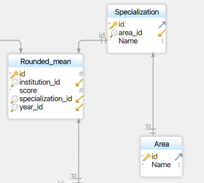
The physical data model looks takes the following shape (with the help of DbSchema) Note that this was just the initial, logical data model. The final version looks like this:
The first part of the process will be creating the database. Once created and populated with all PGR data, I can then begin querying and visualizing it so as to offer analyses. Finally–and this is a bit aspirational–I hope to share the database and create an interface so users can easily access the information they need about e.g., a particular specialization or institution.
The project consists of four main components that will populate the database. First is creating and populating an initial database with the necessary tables to store the overall scores and information for the most recent iteration of the PGR. Second is creating and populating of more tables pertaining to the specialized scores for each institution. Third is adding historical data from previous PGR iterations in both overall and specialized tables. Fourth will be offering analyses based on junction tables, queries, visualizations, and more.
Contents:
- Creating the Database: Overall Scores for 2021
- Creating the Database: Past Overall Scores
- Creating the Database: Specialized Scores
- Known Issues
- Links
Overall Scores Data
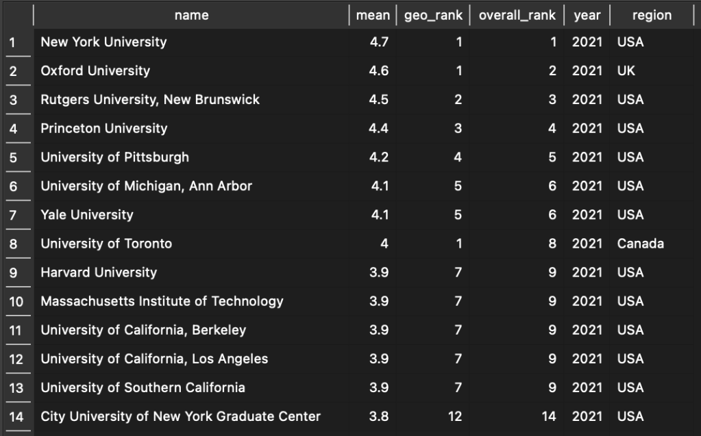
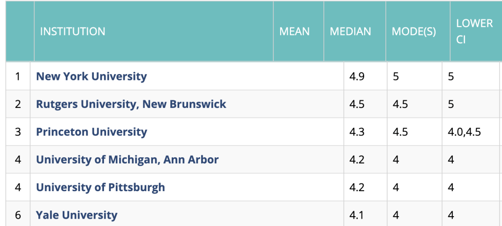
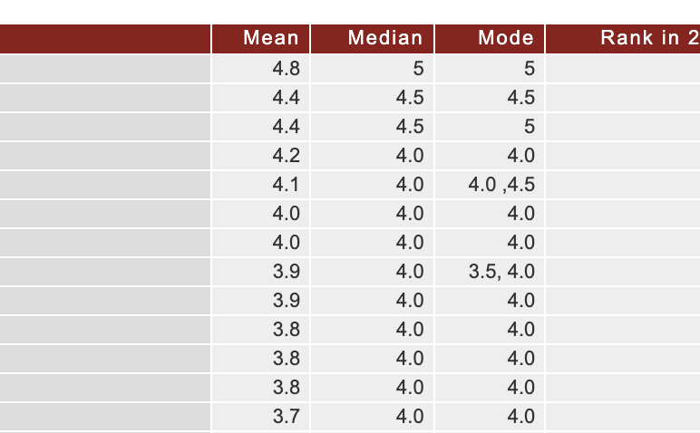
The first step of creating the database is to create CSV files based on the PGR table data for the overall scores and ranks of institutions in the English-speaking world. To do this, I simply copy-and-pasted the data from each table from the PGR Overall Rankings page into an Excel file, like in the screenshot below. A few things to note about this: First, I have ignored the table data about ranks in previous years. This is because I will be using the entire datasets from previous years to populate the database, so there’s no need to include them now. Second, I had to manually enter some of the ranking data into the table, since the overall and regional rankings (“geo_rank” in the table) are on different tables on the PGR Overall Rankings site.

Once I had the CSV file, I had to design a data model to house the data. Using DbSchema, I was able to create a data model for both the Overall and Specialized scores, but the first priority was the Overall scores. The data model looks like this:
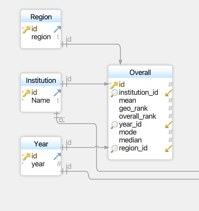
The model is fairly simple, but accomplishes something important: all the data in the “Overall” table is stored as numbers, thus eliminating duplicate strings. Instead of each set of scores being tied to a particular institution’s string name, they point to the id value that serves as the primary key of an Institution table. Ditto for the geographical region and for the year, each of which have their own separate tables.
So once I had the CSV file ready and the data model designed, the task was to write a script that would translate the CSV into the desired data model. The full program I wrote can be found on Github, but I’ll walk through the process here step-by-step.
The first thing I did was import the two required packages: csv and sqlite3, connect to the database, and create the cursor object.
#Import 'csv' to read CSV files and sqlite3 to edit the database
import csv
import sqlite3

#Connect to PGR database
connection = sqlite3.connect('pgr-db-1.db')

# Creating a cursor object to execute
# SQL queries on a database table
cursor = connection.cursor()
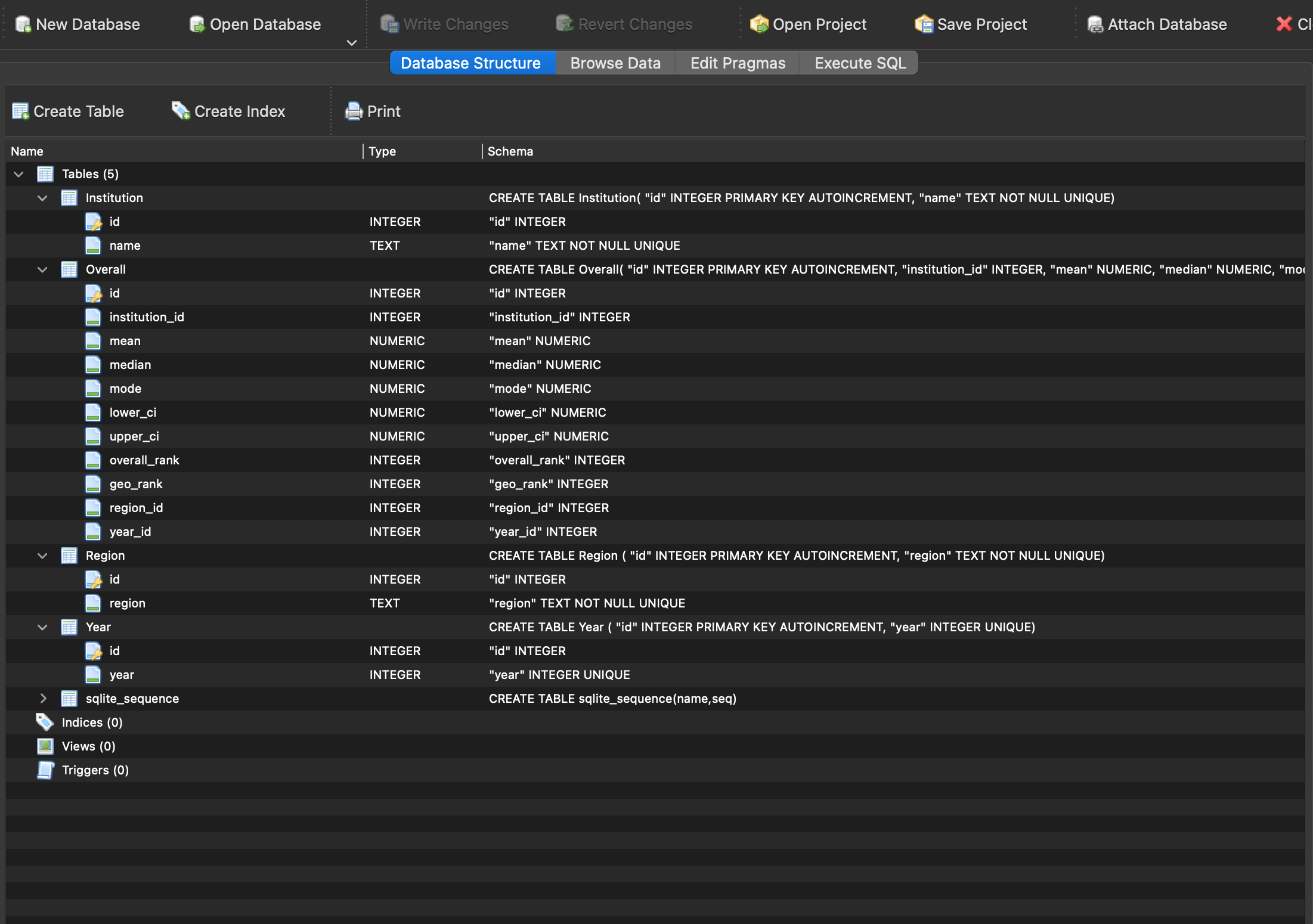
I then wrote the SQL necessary to create the four tables in accordance with the data model above: Institution, Year, Region, and Overall, and executed the commands with cursor.executescript
#Create Institutions Table Overall Table
create_table = '''DROP TABLE IF EXISTS Institution; CREATE TABLE Institution(
                "id" INTEGER PRIMARY KEY AUTOINCREMENT,
                "name" TEXT NOT NULL UNIQUE);

                DROP TABLE IF EXISTS Year; CREATE TABLE Year (
                "id" INTEGER PRIMARY KEY AUTOINCREMENT,
                "year" INTEGER UNIQUE);

                DROP TABLE IF EXISTS Region; CREATE TABLE Region (
                "id" INTEGER PRIMARY KEY AUTOINCREMENT,
                "region" TEXT NOT NULL UNIQUE);

                DROP TABLE IF EXISTS Overall; CREATE TABLE Overall(
                "id" INTEGER PRIMARY KEY AUTOINCREMENT,
                "institution_id" INTEGER,
                "mean" NUMERIC,
                "median" NUMERIC,
                "mode" NUMERIC,
                "lower_ci" NUMERIC,
                "upper_ci" NUMERIC,
                "overall_rank" INTEGER,
                "geo_rank" INTEGER,
                "region_id" INTEGER,
                "year_id" INTEGER);


                '''
cursor.executescript(create_table)
Once the tables were created, I asked the program to prompt for the CSV file. There was only one file to use for now, so I had that one automatically selected unless I typed something different (e.g. for test files).
fname = input('Input CSV file:')
if (len(fname) < 1): fname = 'PGR_COMBINED.csv'

#Open the CSV file
fh = open(fname, newline='')

#Read the CSV file
contents = csv.reader(fh)
I then set my variables to use for the SQL insertions and deletions to populate the tables. Some of these were a bit clunky, especially the deletions, but they get the job done by accomplishing one of three main things: inserting the CSV values into the right tables, deleting the headers from the CSV (which I could have just deleted myself) and any empty rows, and pulling up the id’s based on a name from the Institution, Year, and Region tables.
#Variables for SQL insertion
#Insert values
insert_institution = "INSERT OR IGNORE INTO Institution (name) VALUES ( ? )"
insert_region = "INSERT OR IGNORE INTO Region (region) VALUES ( ? )"
insert_year = "INSERT OR IGNORE INTO Year (year) VALUES ( ? )"
insert_overall = "INSERT OR IGNORE INTO Overall (institution_id, mean, median, mode, lower_ci, upper_ci, geo_rank, region_id, overall_rank, year_id) VALUES ( ?, ?, ?, ?, ?, ?, ?, ?, ?, ?)"

#Delete headers and empties
delete_i_header = "DELETE FROM Institution WHERE name = '\ufeffINSTITUTIONS'"
delete_i_empty = "DELETE FROM Institution WHERE name = ''"
delete_y_header = "DELETE FROM Year WHERE year = 'year '"
delete_y_empty = "DELETE FROM Year WHERE year = ''"
delete_o_header = "DELETE FROM Overall WHERE mean = 'MEAN' "
delete_r_header = "DELETE FROM Region WHERE region = 'REGION'"

#Get IDs for Year, Region, and Institution
get_inst_id = "SELECT id FROM Institution WHERE name = ? "
get_year_id = "SELECT id FROM Year WHERE year = ? "
get_region_id = "SELECT id FROM Region WHERE region = ? "
Next came the execution. With the CSV file now being read as contents, I could now iterate through each row and each item therein which would then fill the “?” characters in the SQL variables. Each row is a list, and each item in the row is a member of that list, which I can then refer to via an index, assigned to a variable, and then called in the SQL command.
#Write rows of CSV to database
for row in contents:
    #Identify row indices
    inst = row[0]
    mean = row[1]
    median = row[2]
    mode = row[3]
    lower_ci = row[4]
    upper_ci = row[5]
    region = row[6]
    geo_rank = row[7]
    overall_rank = row[8]
    year = row[9]
    print(row)
    #Populate institution, year, and region tables
    cursor.execute(insert_institution, ( inst, ) )
    cursor.execute(insert_year, ( year, ) )
    cursor.execute(insert_region, ( region, ))
    #get IDs for Overall table
    cursor.execute(get_inst_id, ( inst, ))
    inst_id = cursor.fetchone()[0]
    cursor.execute(get_year_id, ( year, ))
    year_id = cursor.fetchone()[0]
    cursor.execute(get_region_id, ( region, ))
    region_id = cursor.fetchone()[0]
    #Populate overall tables
    cursor.execute(insert_overall, ( inst_id, mean, median, mode, lower_ci, upper_ci, geo_rank, region_id, overall_rank, year_id ) )
    #Delete headers and nulls
    cursor.execute(delete_i_header)
    cursor.execute(delete_i_empty)
    cursor.execute(delete_y_header)
    cursor.execute(delete_r_header)
    cursor.execute(delete_y_empty)
    cursor.execute(delete_o_header)
connection.commit()
Finally, I checked the results of the insertions:
#Check results of Institution Table
res_i = cursor.execute('''SELECT * FROM Institution LIMIT 10''')
print(res_i.fetchall())
#Check results of Year table
res_y = cursor.execute('''SELECT * FROM Year LIMIT 10''')
print(res_y.fetchall())
#Check results of region Table
res_r = cursor.execute('''SELECT * FROM Region LIMIT 10''')
print(res_r.fetchall())
#Check results of Overall table
res_o = cursor.execute('''SELECT * FROM Overall LIMIT 10''')
print(res_o.fetchall())

connection.close()
The output of these commands can be found on Github just for fun, but a preview of the first 10 rows for each table is below:
[(2, 'New York University'), (3, 'Rutgers University, New Brunswick'), (4, 'Princeton University'), (5, 'University of Pittsburgh'), (6, 'University of Michigan, Ann Arbor'), (7, 'Yale University'), (8, 'Harvard University'), (9, 'Massachusetts Institute of Technology'), (10, 'University of California, Berkeley'), (11, 'University of California, Los Angeles')]
[(2, 2021)]
[(2, 'USA'), (60, 'UK'), (79, 'Canada'), (87, 'Australasia')]
[(2, 2, 4.7, 5, 5, 4.7, 4.8, 1, 1, 2, 2), (3, 3, 4.5, 4.5, 5, 4.4, 4.6, 3, 2, 2, 2), (4, 4, 4.4, 4.5, 5, 4.3, 4.5, 4, 3, 2, 2), (5, 5, 4.2, 4, 4, 4, 4.3, 5, 4, 2, 2), (6, 6, 4.1, 4, 4, 4, 4.3, 6, 5, 2, 2), (7, 7, 4.1, 4, 4, 4, 4.2, 6, 5, 2, 2), (8, 8, 3.9, 4, 4, 3.8, 4, 9, 7, 2, 2), (9, 9, 3.9, 4, 4, 3.8, 4, 9, 7, 2, 2), (10, 10, 3.9, 4, 4, 3.8, 4, 9, 7, 2, 2), (11, 11, 3.9, 4, 4, 3.8, 4, 9, 7, 2, 2)]
It looks like a mess, but it’s exactly what I wanted: Tables for each repeatable string value with id numbers and string values (Institution, Region, Year), and one table with overall score values stored entirely as numbers.
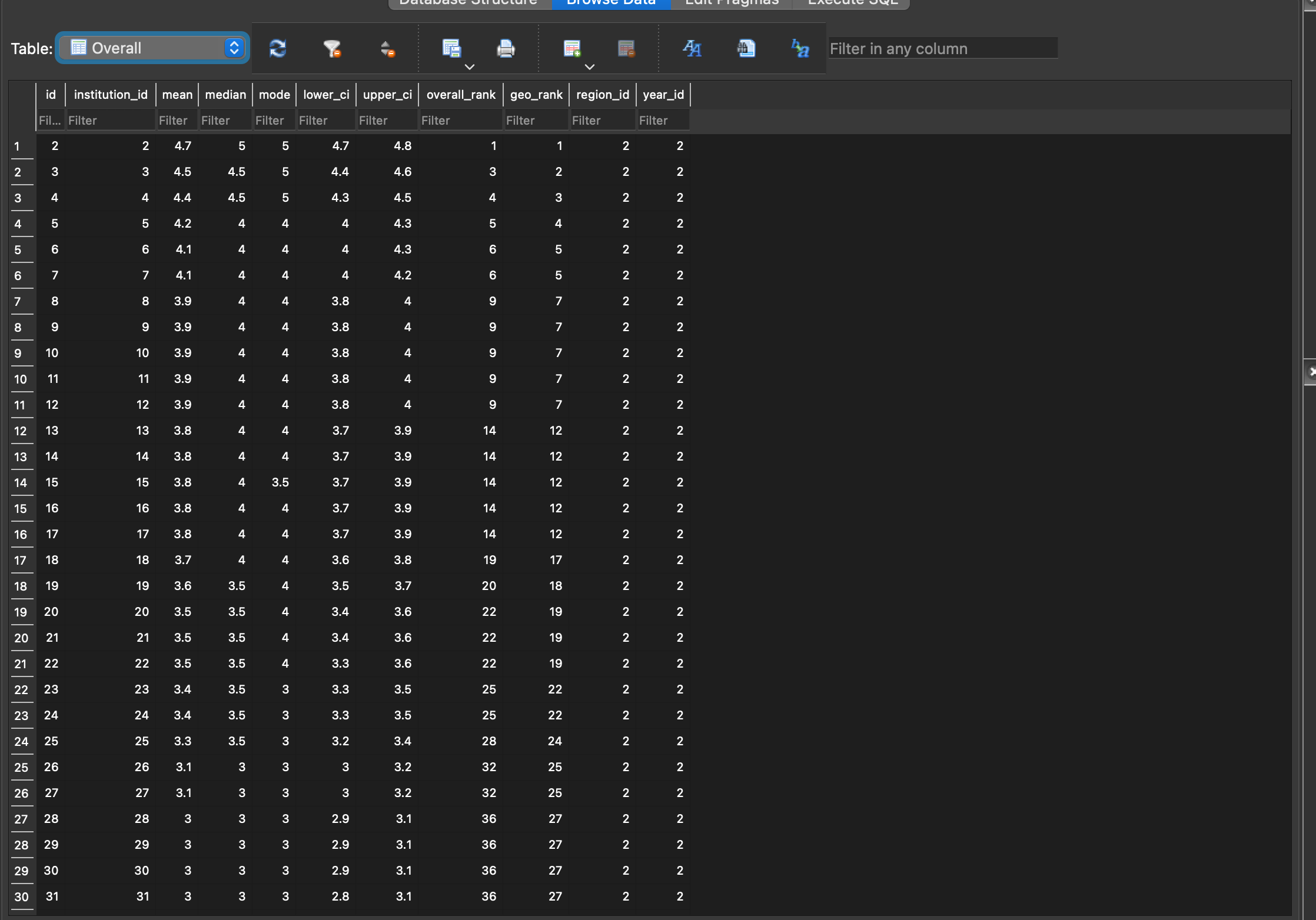
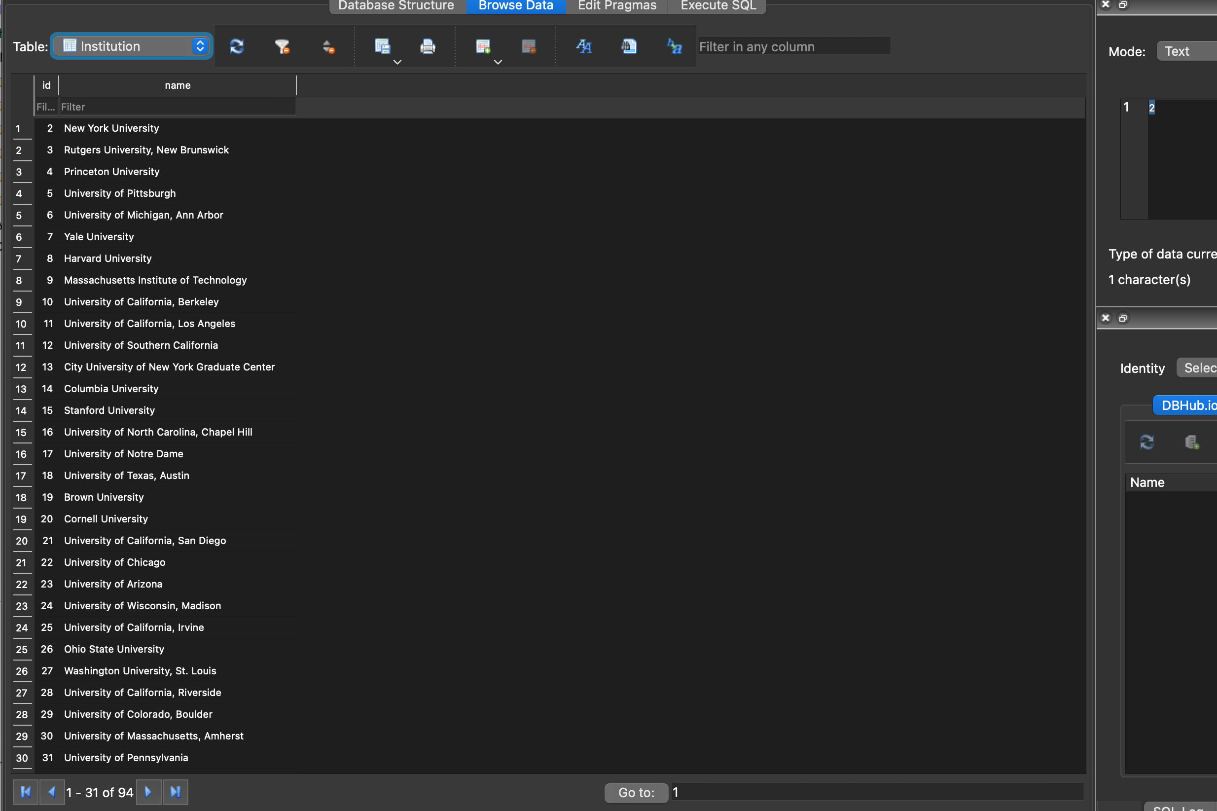
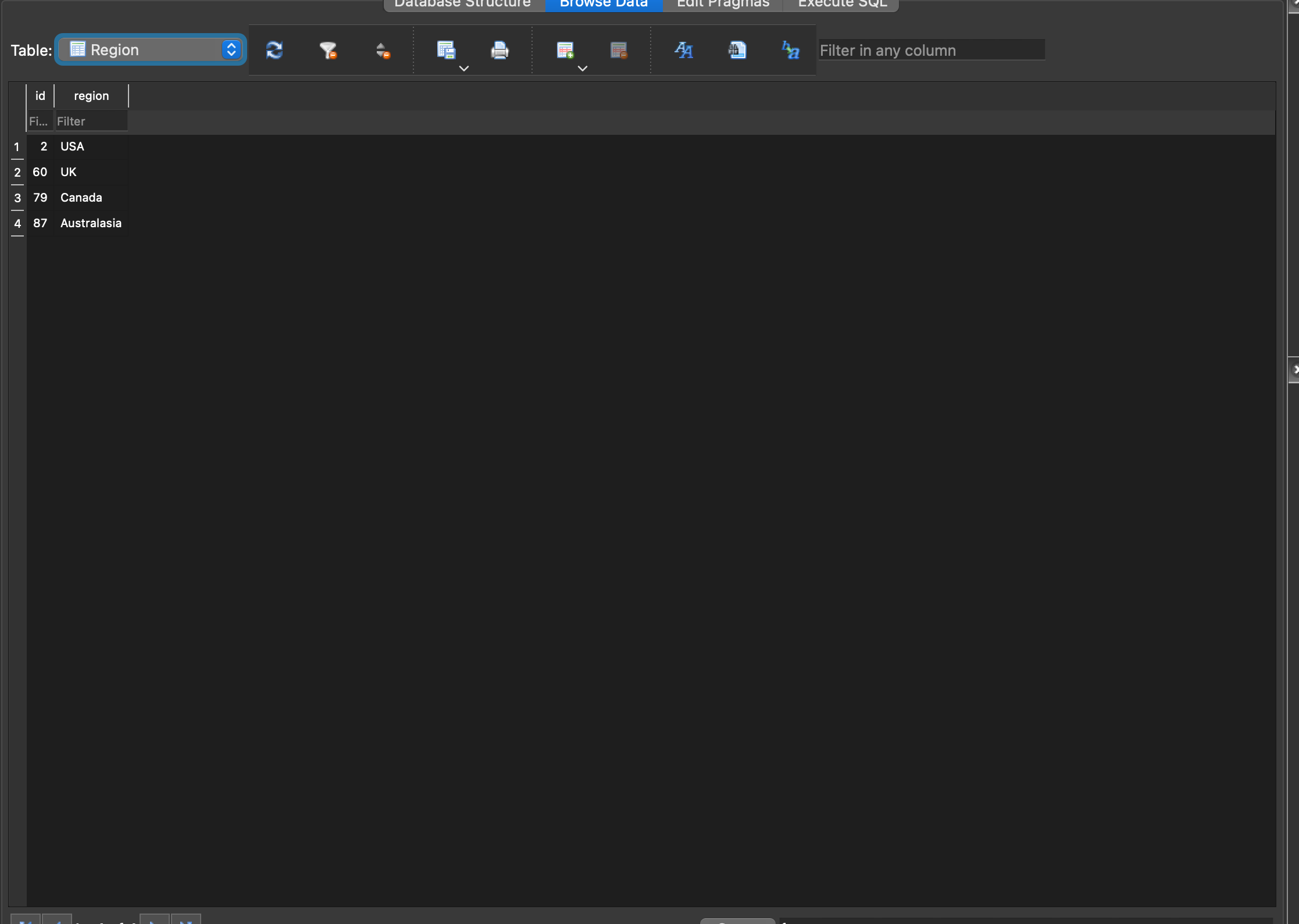
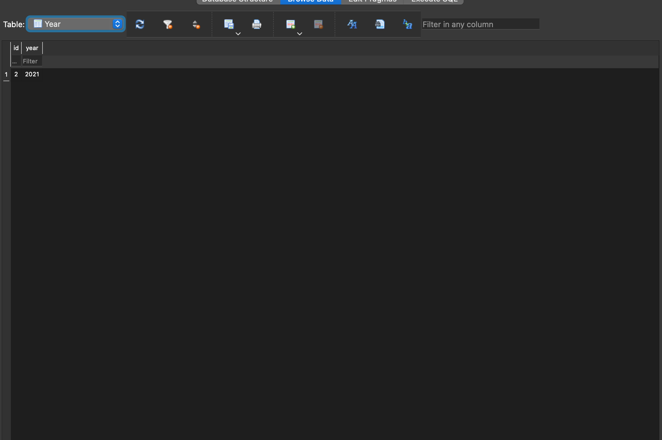
Now we can open the database in a browser, which for me at the moment is DB Browser for SQLite. We can see the database structure below and screenshots of the “Browse Data” tab for each table in the slideshow below:
Finally, we can make the data a bit more useful by essentially getting back to where we started from on the PGR website: A table that displays useful information about each Institution. To do this, we simply need to use some SQL to pull all the relevant data from each table and return the rows and columns we’re interested in. The most basic query would be this:
--Look up all institutions and basic info
SELECT Institution.name, Overall.mean, Overall.geo_rank, Overall.overall_rank, Year.year, Region.region
FROM Institution JOIN Overall JOIN Year JOIN Region
ON Institution.id = Overall.institution_id AND Overall.region_id = Region.id AND Overall.year_id = Year.id
Which returns the institution’s name, mean, rank within its geographical are, overall rank, region, and the year of assessment:
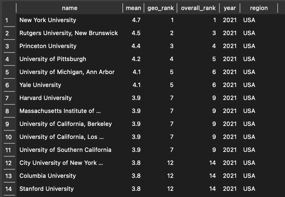
The order here is based on the order of the data, which follows the PGR by listing the US schools first, then the UK, Canada, and Australasia below (not shown). If we wanted to list all the schools by their mean score or rank (which should generate the same results), we just have to add an ORDER BY clause to our query:
--Look up all records and sort by rank
SELECT Institution.name, Overall.mean, Overall.geo_rank, Overall.overall_rank, Year.year, Region.region
FROM Institution JOIN Overall JOIN Year JOIN Region
ON Institution.id = Overall.institution_id AND Overall.region_id = Region.id AND Overall.year_id = Year.id
ORDER BY Overall.mean DESC
This essentially recreates the Overall ranking found on the PGR site, while also displaying Institutions’ regional ranking in the same table. For example, the University of Toronto is ranked 8 overall due to its mean score, but it is ranked 1 in Canada.
So far, we’ve just taken an extremely roundabout way to get back to where we started: a table that lists an Institution’s name, scores, rank, and geography, just like the one found on the PGR Website. But as a first step in the project, this is a good thing! Under the hood of this intuitive table, we have a flexible data model that we can now add to and rely on for more advanced queries and eventually visualizations. But first, we need to add more data!
Creating the Database: Past Overall Scores
Modifying the elements above to include historical data was, well, trivial from a coding perspective. All I needed was a CSV file containing all the relevant data for each iteration of the PGR and the Python script did the rest, creating and occupying the tables with the relevant data for each year: 2021, 2017, 2014, 2011, 2009, and 2006. I decided to stop at 2006 because, well, I can’t find the page for the 2004 report. Plus, in 2006, there were no schools included from Australasia, nor was there an overall rank for institutions, so it seems like 2006 was the first year that the PGR took the the shape it would maintain until the 2017 report. There are other idiosyncrasies about the data, but at least we have mean scores and regional ranks for each top institution from 2006-2021.
As for creating the database, I wasn’t entirely sure of using a single CSV instead of one for each year. On the one hand, it seems a bit neater to have a different CSV file for each year. On the other hand, it seems far easier to have them all be in one file with enough fields (namely, the “Year” field) to differentiate each entry. All the data ends up in the same place anyway, and I don’t have to worry about getting rid of column headers for each file, which brings me to the next issue…
While the scripting was easy, the bigger task was cleaning the data, since the older iterations of the PGR were presented in a different format, and there were some quirks. For example, some Institutions had slightly different names in older versions of the report. For example, “University of St. Andrews/University of Stirling Joint Program” was shortened in 2017 to “University of St. Andrews/Stirling Joint Program.” Elsewhere, some schools had smart and un-smart apostrophes (“Queen’s University, Kingston” vs. “Queen’s University, Kingston”), spaces before commas (“Rutgers University , New Brunswick” vs. “Rutgers University, New Brunswick”), and even typos! (The 2014 PGR misspells “Massachusetts” as “Massachussetts” a couple of times.) Another issue was that in earlier iterations of the report, some institutions had two “mode” scores. In such cases, I just deleted both of them, since what it means is that two scores were equally common. Most institutions only had one mode score so I only had to do this in three cases (I believe).
Here are the links to the PGR Overall rankings from each year for you to see for yourself:
At the end of it all, I was left with a cleaned CSV file with the relevant data for each Institution from 2006 to 2021 including the institution name, mean score, geographical rank, overall rank, and the year. median, mode, upper CI, lower CI, region, and year—at least where the PGR supplies values. You can view and download the file on my Kaggle page.
Upon running the Python script above, we are left with the following familiar preview:
[(2, 'New York University'), (3, 'Rutgers University, New Brunswick'), (4, 'Princeton University'), (5, 'University of Pittsburgh'), (6, 'University of Michigan, Ann Arbor'), (7, 'Yale University'), (8, 'Harvard University'), (9, 'Massachusetts Institute of Technology'), (10, 'University of California, Berkeley'), (11, 'University of California, Los Angeles')]
[(2, 2021), (96, 2017), (187, 2014), (281, 2011), (368, 2009), (467, 2006)]
[(2, 'USA'), (60, 'UK'), (79, 'Canada'), (87, 'Australasia')]
[(2, 2, 4.7, 5, 5, 4.7, 4.8, 1, 1, 2, 2), (3, 3, 4.5, 4.5, 5, 4.4, 4.6, 3, 2, 2, 2), (4, 4, 4.4, 4.5, 5, 4.3, 4.5, 4, 3, 2, 2), (5, 5, 4.2, 4, 4, 4, 4.3, 5, 4, 2, 2), (6, 6, 4.1, 4, 4, 4, 4.3, 6, 5, 2, 2), (7, 7, 4.1, 4, 4, 4, 4.2, 6, 5, 2, 2), (8, 8, 3.9, 4, 4, 3.8, 4, 9, 7, 2, 2), (9, 9, 3.9, 4, 4, 3.8, 4, 9, 7, 2, 2), (10, 10, 3.9, 4, 4, 3.8, 4, 9, 7, 2, 2), (11, 11, 3.9, 4, 4, 3.8, 4, 9, 7, 2, 2)]
This looks right! The main difference between this and the previous one is that our “Year” table has multiple entries for each year of the report, which is exactly what we want. Our Overall table looks the same too, only now we have entries corresponding for different years, which we can see here:
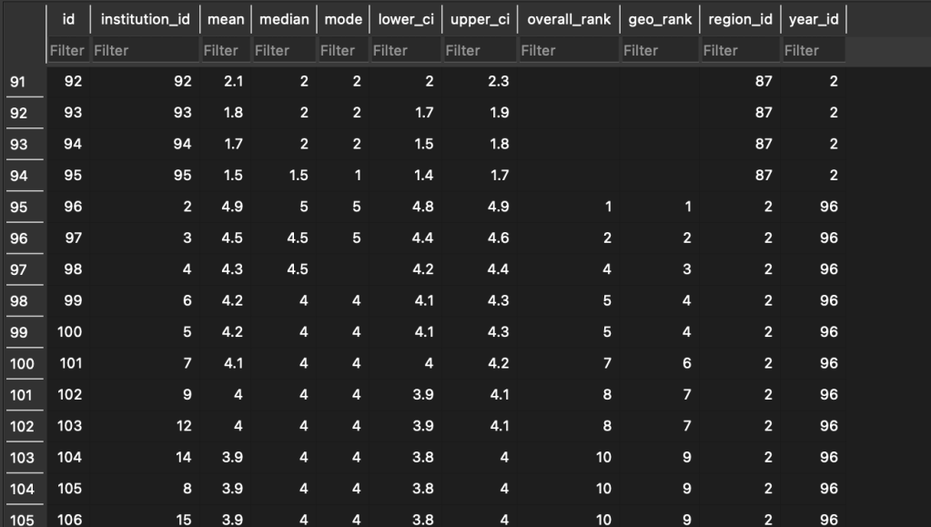
On row 95, the year_id changes to 96, which is the id for 2017. Now we know that everything that follows is from the 2017 report. We also know that we’re at the top of the report because the institution_id has been changed to 2, which is the code for New York University, whose overall_rank and geo_rank are both 1.
With the database populated with PGR data on overall scores from 2006-2021, and all repeating strings changed to numbers pointing to primary key values in other tables, we’re now ready to start performing some interesting queries and even creating some visualizations based on this data! I’ll have a whole section on different queries a reader might want to run for analyzing this data, but for now I just want to showcase one crucial and useful query we can now run: an institution’s change in rank and score over time. For example, to see how Duke University has fared over the years, we run the following query:
--Look up a particular school by name.
SELECT Institution.name, Overall.mean, Overall.geo_rank, Overall.overall_rank, Year.year, Region.region
FROM Institution JOIN Overall JOIN Year JOIN Region
ON Institution.id = Overall.institution_id AND Overall.region_id = Region.id AND Overall.year_id = Year.id
WHERE Institution.name = "Duke University"
And get the following result:
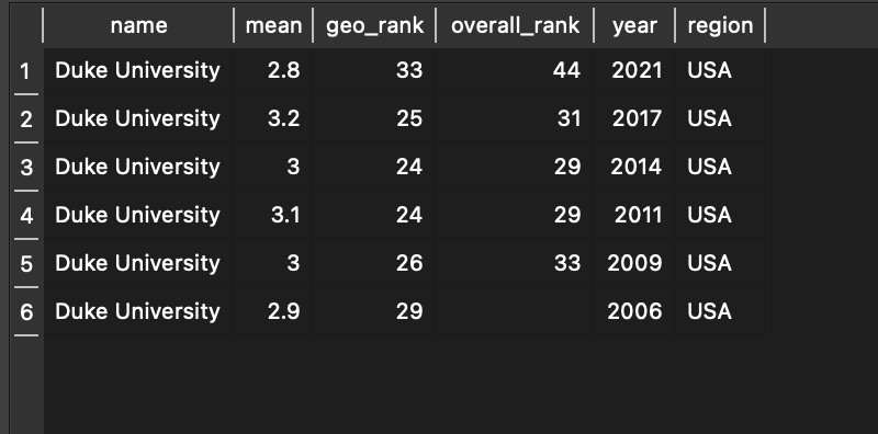
We can see that, at a glance, Duke’s rank and mean score in 2021 is lower than it was in 2006. Its mean score peaked in 2017, but its rank peaked in 2011 and 2014. We can run this query for any institution we like to see how its scores have changed over time, and we can choose which data we want to see about it.
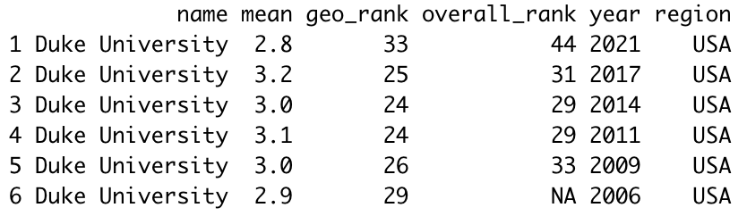
Finally, using DB Browser for SQLite, we can export the table above as a CSV file that we can examine using R. Once we load the file as a dataframe, the head() command gives us the following:
We can then use ggplot2 to plot the mean score over time:
ggplot(data=duke_scores, aes(x=year, y=mean)) +
  geom_line(color="red")+
  geom_point()+
  coord_cartesian(ylim = c(1, 5)) +
  labs(title="Duke University Mean Score over Time")
This gives us the following result:
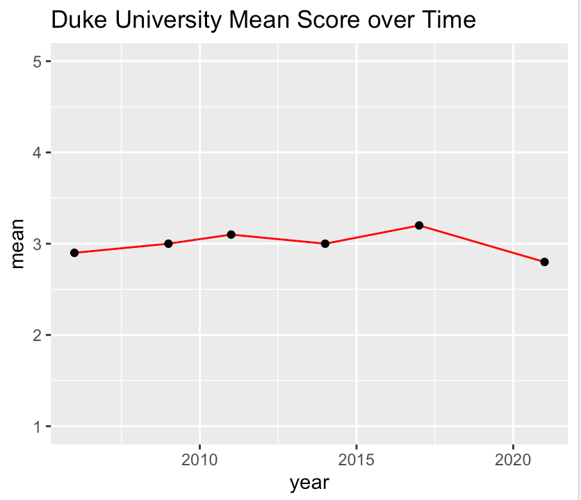
We can now see quite easily how Duke University’s mean score has changed over time, and all it took was a basic query of our database and a very quick R script to generate. We can now perform the same functions for any institution and any data point.
These are just some of the most basic functions we now have access to with our new PGR database, and it should be easy to see how they can combine to generate some more powerful visualizations and queries to help us better understand and analyze the full dataset.
Creating the Database: Specialized Scores
Creating the specialized scores in the database required a bit more effort because the dataset is much larger. Additionally, the data is spread out over multiple tables on different PGR websites, and the format was inconsistent, which in turn increased the risk of typos and other data dirtiness.
The first thing I had to do was decide on the data model. I ended up adding 3 tables to the database: one for the scores, one for the specializations, and one for the areas.
To gather the data, I decided to write a web scraper with Python to copy the HTML from each of the specialty pages on the PGR sites, since in earlier iterations of the PGR, each specialization had its own page! Mercifully, from 2009-2014, the specialty scores were all on a single page, which made things considerably easier.
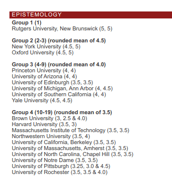
I then had to parse the HTML, which was a bit of a pain. The names of the specialties were in all caps, and the HTML for each year was a bit different. Additionally, the values for median and mode were placed in parentheses next to the institution name in each table, the group and mean scores were placed at the top of the table rather than in each entry row, and some institutions had multiple mode values:
I used a Python script to parse the HTML and generate rows to be written in the CSV file. I first made a list titled row with placeholder data and then an empty list called allrows. I then defined a series of functions utilizing regular expressions to pull the relevant data from the rows of HTML, and then passed them through a for loop that generated entries to be added to row. The finished row would then be added to allrows, which would then be written to the CSV. The items in row would only update if the function succeeded, and would otherwise be left alone, enabling me to automatically duplicate the area, specialization, group, and mean score entries for different institutions until a new one appeared in the next table or group.
#The for loop to make it all work:

for line in fh:
    line = line.lstrip()
    try:
        get_area()
    except:
        pass
    try:
        get_specialization()
    except:
        pass
    try:
        get_group_and_mean()
    except:
        pass
    try:
        get_median_and_name1()
    except:
        pass
    try:
        get_median_and_name2()
    except:
        pass
    if line.startswith('<p class="MainTxtJust"><strong>Also'):
#        #gets rid of entry for this line
       allrows.pop(-1)
#        break
Each iteration of the PGR had its own CSV file, which I then manually combined and cleaned, removing misspelled university names (e.g., “University of Read”, and lots of “Massachussetts”), before it was ready to be entered into the database.
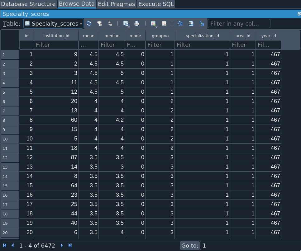
I then had to enter the data into the database using a new database writer script that generated the three necessary tables. It would also look up the ID number for each institution and year. (I’ve now realized that the “year” table is totally redundant, since there’s no need to keep a second table for integer values. Perhaps I’ll fix this someday.) The result is 3 new tables: Area, Specialization, and Specialty_scores:
Most impressive is the Specialty_scores table, which boasts 6472 lines of data. Granted, that’s precisely the size of the CSV file, but here it is in database form, no strings attached.
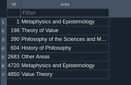
After the database was created, I also had to do some cleaning of the CSV files, mostly with checking the Institution names. The Specialization names also proved a bit troublesome, since those often changed over time. For example, in 2006 and 2008, Normative Ethics and Moral Psychology were grouped together, but from 2017, Metaethics and Moral Psychology have been combined. You can see other such idiosyncrasies below:
In cases where the variations were merely typographical (e.g., “19th-century” vs “19th Century”), I standardized the specialization entry. In cases where the differences appeared substantive (e.g., whether Moral Psychology is grouped with Normative Ethics or Metaethics), I left the original categories. There were some difficult cases are where I had to make an executive decision, e.g., changing “Philosophy of Science”, the specialization title from 2006-2008, to “General Philosophy of Science”, which was implemented from 2011 onward. The titles of the major Areas of philosophy tended to stay the same over time.
And that’s it! Now we can start to examine the specialization data in more detail and run queries to pull up and visualize the data we need. For example, suppose we want a list of all the specialties of a certain institution (e.g., University of Toronto) ranked by specialization mean score:
SELECT Institution.name, Specialization.specialization, Specialty_scores.mean, Specialty_scores.groupno, Year.year
FROM Institution JOIN Specialization JOIN Year JOIN Specialty_scores JOIN Area
ON Institution.id = Specialty_scores.institution_id
AND Specialty_scores.area_id = Area.id
AND Specialty_scores.specialization_id = Specialization.id
AND Specialty_scores.year_id = Year.id
WHERE Institution.name = "University of Toronto" AND Year.year = 2021
ORDER BY Specialty_scores.mean DESC
This gives us the following results:
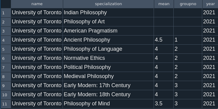
Indian Philosophy, Philosophy of Art, and American Pragmatism lack groupings or mean scores in 2021, but University of Toronto is still recommended for those programs. Its most highly rated specializations are listed from rows 4-10, with its strongest specialization being in Ancient Philosophy. Four out of seven of its highest rated specializations are in the History of Philosophy, a conclusion easily drawn from this query that might be useful to students looking to specialize within the History of Philosophy.
If we want to see how the University of Toronto’s score for Ancient Philosophy has changed over time, we just need to eliminate the year specification in our WHERE clause and add one that specifies “Ancient Philosophy”, giving us the following results:
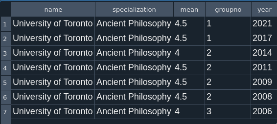
Thus we can conclude that the University of Toronto has had consistently strong scores in Ancient Philosophy since 2006.
Final Database Model
And thus, the database is complete. The final data model looks like this:
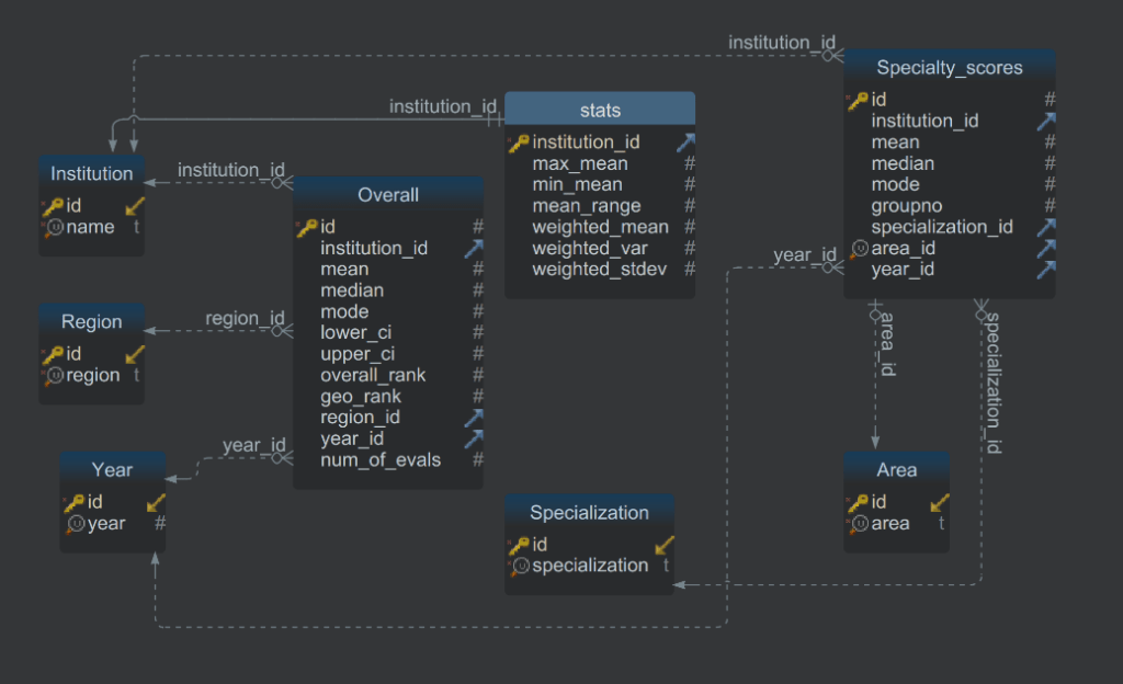
The database is fully relational, with no duplicate strings. It contains a table with overall data, summary statistics, and specialty score data. Now, all it needs is a UI.
Known issues
- Median and Mode score data is limited for previous iterations, including 2017.
- There may be typos and errors in the data itself, especially in Institution names.
- The “year” table is redundant.
